Tutorial Step 2: What's in a LIGO Data File?

In this tutorial, we will use Python to read a LIGO data file. If you don't have an HDF5 LIGO data file stored on your computer somewhere, go back to Tutorial Step 1. If you do not have Python or some of the needed modules installed on your computer, go back to Tutorial Step 0.

Start the Python Interpreter

Writing a Python script has two parts:

• The .py file, which is your code, and should be created with a text editor such as emacs or vi. If you installed Enthought Canopy, this should come with its own text editor.
• The Python interpreter, that executes the code

To get started, try to open the Python interpreter. This will be a little different on different platforms. If you installed Canopy, then click the Canopy icon from wherever you usually run applications (for example, the Windows start menu, or the Mac Applications directory). If you installed using MacPorts, try this command in the terminal window:

/opt/local/bin/python2.7

Similar commands should work for users of other Unix-like systems. You should see something along these lines:

Python 2.7.3 (default, Nov 17 2012, 19:54:34) 
[GCC 4.2.1 Compatible Apple Clang 4.1 
((tags/Apple/clang-421.11.66))] on darwin
Type "help", "copyright", "credits" or "license" 
for more information.
>>> 

You can exit out of Python by typing

>>> exit()

Let's try to write a very simple program. Move into the directory where you placed your LIGO data file. Now you should open two windows at the same time: the Python interpreter window and a text editor window where you can see the contents of a new text file, which we'll call plot_strain.py. Canopy shows both windows by default - just create a new file called plot_strain.py. On a Mac or Unix machine, do something like this:

$ cd ~/ligoData
$ emacs plot_strain.py &
$ /opt/local/bin/python-2.7

Now, in the plot_strain.py file, add the following text:

print "Hello, world!"

and save the file. Then, in the python interpreter window, you can run the entire contents of plot_strain.py by typing:

>>> import plot_strain 

Or, if you are using IPython and/or Canopy, you should be able to use the magic command run instead:

In [1]: run plot_strain

If all goes well, you'll see the text Hello, world! appear in your interpreter window.

Data File Overview

Let's try to read in and plot some LIGO data. In plot_strain.py, let's remove the code print "Hello, world!" and replace it with:

#----------------------
# Import needed modules
#----------------------
import numpy as np
import matplotlib.pyplot as plt
import h5py

This will tell Python that we want to use the numerical Python (numpy), HDF5 module (hypy), and plotting module (matplotlib.pyplot). We'll always put this at the top of the scripts we write in this tutorial.

Next, try reading in the LIGO data file that you downloaded in the last step of this tutorial.

#-------------------------
# Open the File
#-------------------------
fileName = 'H-H1_LOSC_4_V1-815411200-4096.hdf5'
dataFile = h5py.File(fileName, 'r')

dataFile is now an object which can be treated as a Python dictionary, and contains all of the information from the data file. To get an idea of what's in the file, add this code to plot_strain.py:

#----------------------
# Explore the file
#----------------------
for key in dataFile.keys():
    print key 

Trying running this code in the interpreter. You can use the command import plot_strain or reload(plot_strain) if you have already imported a previous version of the file. If you are using IPython, you can also use the command run plot_strain instead. You should see something like this:

>>> reload(plot_strain)
meta
quality
strain

This gives a high level picture of what's contained in a LIGO data file. There are 3 types of information:

• meta: Meta-data for the file. This is basic information such as the GPS times covered, which instrument, etc.
• quality: Refers to data quality. The main item here is a 1 Hz time series describing the data quality for each second of data. This is an important topic, and we'll devote a whole step of the tutorial to working with data quality information.
• strain: Strain data from the interferometer. In some sense, this is "the data", the main measurement performed by LIGO.

For a general introduction to gravitational waves and measurements made by LIGO, we suggest reading articles or watching videos available on ligo.org.

Plot a time series

Let's continue adding to plot_strain.py to make a plot of a few seconds of LIGO data. To store the strain data in a convienient place, add these lines to plot_strain.py

#---------------------
# Read in strain data
#---------------------
strain = dataFile['strain']['Strain'].value
ts = dataFile['strain']['Strain'].attrs['Xspacing']

The code above accesses the 'Strain' data object that lives inside the group 'strain'. The "attribute" 'Xspacing' tells how much time there is between each sample, and we store this as ts. The "value" of the data object contains the strain value at each sample - we store this as strain. To see all the structure of a GWOSC data file, take a look at the View a File tutorial.

Now, let's use the meta-data to make a vector that will label the time stamp of each sample. In the same way that we indexed dataFile as a Python dictionary, we can also index dataFile['meta']. To see what meta-data we have to work with, add these lines to plot_strain.py:

#-----------------------
# Print out some meta data
#-----------------------
print "\n\n"
metaKeys = dataFile['meta'].keys()
meta = dataFile['meta']
for key in metaKeys:
    print key, meta[key].value

In the python interpreter, enter reload(plot_strain) to see the output of this. You should see that the GPS start time and the duration are both stored as meta-data. To calculate how much time passes between samples, we can divide the total duration by the number of samples:

#---------------------------
# Create a time vector
#---------------------------
gpsStart = meta['GPSstart'].value
duration = meta['Duration'].value
gpsEnd   = gpsStart + duration

time = np.arange(gpsStart, gpsEnd, ts)

The numpy command arange creates an array (think a column of numbers) that starts at gpsStart, ends at gpsEnd (non-inclusive), and has an increment of ts between each element.

Finally, let's use all of this to plot a few seconds worth of data. Since this data is sampled at 4096 Hz, 10,000 samples corresponds to about 2.4 s. Add the following to plot_strain.py

#----------------------
# Plot the time series
#----------------------
numSamples = 10000
plt.plot(time[0:numSamples], strain[0:numSamples])
plt.xlabel('GPS Time (s)')
plt.ylabel('H1 Strain')
plt.show()

The last command, plt.show(), may not be necessary if you are working in the matplotlib interactive mode. You can turn on interactive mode with the command plt.ion().

Now, in the interpreter window, type reload(plot_strain) or run plot_strain and you should see a plot that looks like this:

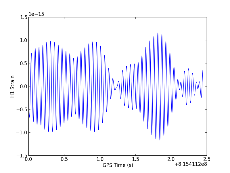
You may be surprised that the data looks smooth and curvy, rather than jagged and jumpy as you might expect for white noise. That's because white noise has roughly equal power at all frequencies, which LIGO data does not. Rather, LIGO data includes noise that is a strong function of frequency - we often say the noise is "colored" to distinguish it from white noise. The wiggles you see in the plot above are at the low end of the LIGO band (around 20 Hz). In general, LIGO noise is dominated by these low frequencies. To learn more about LIGO noise as a function of frequency, take a look at the plot gallery.

• Click here to download the entire script described in this tutorial.

What's next?

• You may want to see the whole structure of a LIGO data file
• Go on to the next part of this tutorial: Step 3: Working with Data Quality