Find a Hardware Injection: Step 1

Introduction

The LIGO data contains simulated signals known as hardware injections. For documenation on hardware injections, see links on the data quality page. This tutorial is based on work by Ashley Disbrow, and will focus on S5 CBC hardware injections, However, many of the techniques shown here can be applied to other types of injections as well.

Using the documentation

Let's start by using the available documentation to pick a hardware injection we want to recover. From the S5 CBC hardware injection page, follow the link to the table of injections for H1. We'll pick an injection with a relatively high SNR for the tutorial. Scroll down until you see GPS time 817064899. You should see a line in the table that looks like this:

817064899 	H1 	10 	10 	25 	Successful 	28.16 	26.55 

This is a simulated black hole/black hole merger, each 10 solar masses, placed at a distance of 25 Mpc from earth. The injection seems to have worked, and was recovered with a signal-to-noise ratio (SNR) of 26.5 using a low-resolution PSD. We're going to emulate that result. However, this tutorial will use a higher resolution PSD, so we should expect to recover the signal with a higher SNR.

We can also look at this time on a timeline, to confirm that the injection is marked in the segment information: (link to timeline). You should be able to see that the injection is present in H1 and H2, but not in L1.

Download the data file

If you do not already know how to download and read a LIGO data file, you may want to start with the Introduction to LIGO Data Files. As a reminder, to download this data file, follow the menu link to Data & Catalogs to find the S5 Data Archive.

• Navigate to the S5 Data Archive
• Select the H1 instrument
• Input the injection time as both the start and end of your query.
• Click submit

This should return a result with only the data file containing the injection.

Find the injection segment

We'll use to open this file, a sample API described in the introductory tutorials.

import numpy as np
import matplotlib.pyplot as plt
import matplotlib.mlab as mlab
import readligo as rl

strain, time, dq = rl.loaddata('H-H1_LOSC_4_V1-817061888-4096.hdf5')
dt = time[1] - time[0]
fs = 1.0 / dt
print dq.keys()

Notice that one of the data quality channels is HW_CBC. Let's plot this channel, and check that there is good data around the injection time using the DEFAULT channel.

plt.plot(dq['HW_CBC'] + 2, label='HW_CBC')
plt.plot(dq['DEFAULT'], label='Good Data')
plt.xlabel('Time since ' + str(time[0]) + ' (s)')
plt.axis([0, 4096, -1, 6])
plt.legend()
plt.show()

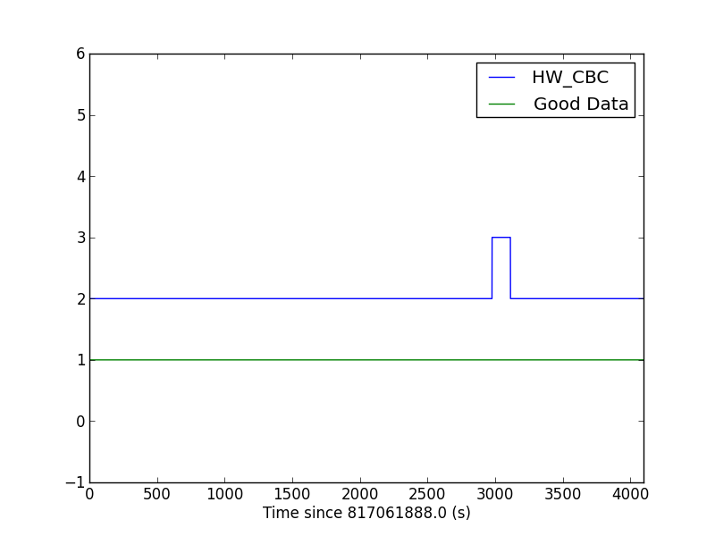
Notice that all the time around the injection passes the default data quality flags (DEFAULT is 1), so we should have no problems analyzing this time.

Finally, let's grab the segment of data containing the injection. We'll also identify a segment of data just before the injection, to use for a PSD estimation. We'll call this the "noise" segment, and it will be 8 times as long as the segment containing the injection.

# -- Get the injection segment
inj_slice = rl.dq_channel_to_seglist(dq['HW_CBC'])[0]
inj_data = strain[inj_slice]
inj_time = time[inj_slice]

# -- Get the noise segment
noise_slice = slice(inj_slice.start-8*len(inj_data), inj_slice.start)
noise_data = strain[noise_slice]

# -- How long is the segment?
seg_time = len(inj_data) / fs
print "The injection segment is {0} s long".format(seg_time)

Running this code should print out that the injection segment is 136 seconds long. We'll search this segment for the signal.

What's next?

Go on to step 2 of this tutorial.